

When you shoot film you have to be an artist and a technician at the same time. Before you open the shutter there are composition, creative use of contrasts and colours, and trickery with lights to be concerned with. After that come the concerns about aperture, shutter speed and film reciprocity behaviour. And then, in the end, there is film development. What developer do you use? At what dilution? And then, for how long do I leave it in? Should I agitate or not? If so, how often? In this article, I will be taking you away from the manuals that come with the developer and film and be showing you one method of determining the film speed and development times that fit your procedures. If you are reading this then there will probably be a lot of new material, so bear with me as I take you through the steps.
Why not stick to what it says on the box? I hear you ask. That is indeed a good question. Film manufacturers have put a lot of effort and consideration in coming up with development methods that will give good results the majority of the time. They quote development times, how to correct for non-ideal temperatures of the chemicals, how to push and pull a film, and even how to change the development times if you are using other development methods (small spiral tank, big dip-dunk system, rotary processing, etc). They have to. If their products were difficult to work with, there would be very little money to be made.
So why deviate from this? Because we want and need to know our materials and methods thoroughly, so that we know what they can do, and eventually don’t have to worry about it anymore. When shooting negative film, the exposure is just the first step. The final image has to be realized in terms of a print or as a scan. We want to make sure we get a negative that is perfect for our needs later on, and one captures all the important information in a format that translates well onto paper. With this in mind, let us start.
To illustrate the methods, I will show you the (intermediate) results of my attempt at characterizing Ilford FP4+, but it will easily apply for other films as well. The procedures below can also be found in Beyond Monochrome (2e) by Lambrecht and Woodhouse in the chapter titled “Customizing Film Speed and Development” and in Beyond the Zone System by Phil Davis. Lambrecht and Woodhouse outline three ways of finding the effective film speed and development time: a quick and easy rule of thumb (will be briefly discussed below), a fast and practical test you can do without a densitometer, and the full densitrometric approach that requires plenty of tests and a densitometer. Phil Davis also discusses the densitometric approach, but includes instructions on how to fancy your own densitometer from a spot meter. In this article, I will be taking the densitometric path, even though most of you will not have the required equipment. I think it will be instructive nonetheless and in an upcoming article I will describe how to make the required equipment yourself without a spot meter.
The Zone System
When talking about densitometry and film testing, there is no way around the “zone system”. Even if you try to run away from it, there will be someone else that brings it up. Tons of books have been written on the topic, some of which are very good, and others are better left on the shelves. I will leave the teaching of the zone system to others, but allow me to elaborate a bit on the topic, to make sure we are all on the same page.
When photographing an arbitrary scene, we try to capture the variations of luminance. This is a technical way of saying there will be different amounts of light coming from different directions. Or even simpler: there will highlights, mid tones and shadows. The difference between the brightest part of the scene and the darkest part (the subject brightness range) can be as high as 10 stops (think bright sunny day in the Sahara) or as low as perhaps 2 or 3 stops (a foggy morning on Loch Ness). Our task as photographers is to make sure all these scenes register on the negative such that they can be printed on paper when we make a print in the darkroom.
Modern negative material has a very large dynamic range (the difference between the darkest and lightest parts it can register at the same time) and therefore most scenes you will encounter will not pose any problems for the film. However, printing paper has a relatively limited dynamic range of approximately 7 zones. By changing our exposure settings and development, we can make sure we utilize the full range of the paper, regardless whether the scene we try to capture spans 3 or 10 zones. This is also important if you are scanning your negatives rather than printing them in the darkroom. The sensors in your scanner have a limited dynamic range that it can cope with also.
To illustrate how this works, lets perform a little thought experiment. We have just exposed some film of an average scene (7 zones between the important shadows and highlights), and are about to develop it. We have mixed the chemicals according to the instructions, and it is even at the suggested temperature of 20 C. So far so good. We pour the developer into the tank and start the clock. As soon as the chemicals get in contact with the emulsion, a reduction reaction converts the latent image into a visible one. In areas where there is a lot of silver nuclei embedded in the grains (the parts that received a lot of light during exposure), this process will go the quickest while in areas that have received little light, the process is less effective. When our timer rings, we pour out the developer and in goes the stop bath to halt the development quickly. As I described in an earlier article, the development time and our agitation interval determine how effective the latent image is converted into a visible one. If we extent our development time, the highlights will continue to develop as there is plenty of nuclei left to convert into silver grains, while at some point the shadows will stop developing, as there are no nuclei available anymore to convert. The longer we develop, the higher our contrast will be.
Now, lets reverse the situation. Instead of varying the development time, we have several sheets of film of the same scene in the same tank, but all sheets have been exposed differently. One of the sheets is severely underexposed, one of them is “correctly” exposed and yet another one is severely overexposed. If we think back of what happens during development, the severely unexposed sheet will have a very faint latent image embedded in the grains. In our limited development time, the grains will only slowly be converted into a visible image and the result will be a nearly transparent sheet with a very faint image present. The highlights will be barely visible, and we have completely lost the shadows. There were so little nuclei available, that locally no visible image could develop. The severely overexposed sheet, on the other hand, will develop very quickly, and look very dense in the end. Perhaps it will appear to be almost opaque to the eye. Our shadows will be clearly visible, and our highlights will be so dense that they are hard to print with any reasonable exposure time.
By controlling the exposure we can make sure that the shadows receive sufficient light so that they will be clearly visible after development, while with our development time we can control the overall contrast of our negative and tame our highlights. Or as others have put it “expose for the shadows, and develop for the highlights”. In the next section, we will take this old adage one step further.
What do we need
When we test film, we want to establish two things: how does development time affect the contrast of our negatives, and how should we expose to make sure all details register correctly? For this we need a few things. First we need a sample of known relative luminance values. We will make identical exposures of this sample when it is evenly illuminated from behind using for example a light box, and develop it for different times. When we then measure the densities of all strips, we can find a relation between relative exposure and density as function of the development time. Second, we will need a tool to measure the resulting densities and we will need a 18% gray card.
I suggest you get a transmission step wedge from Stouffer. Make sure the wedges are at least 3 mm wide, as you will need sufficient real estate during the densitometry. I personally got the T2115 which has 21 wedges, covers a full 10 stops in half stop intervals and nicely fits on a sheet of 4×5 film. You can buy it from Stouffer directly, or via online retailers such as Foto Impex in Berlin for less than 20 euro. If you want to use it to calibrate your densitometer get the calibrated version, otherwise the non calibrated one will be fine, because we will measure the actual densitities ourselves anyway. You will also need a 18% gray card. It is preferably that you get bigger one, such as the B.I.G. Kodak Gray card of 20×25,4 cm for roughly 25 euro. Which leaves the most important bit of kit: the densitometer.
The test requires that you have a transmission densitometer of some sort. Professional models were sold new for several thousand euros years ago, and are still made today by manufacturers like X-Rite. A new one by Heiland (aimed at amateurs) retails new for roughly 700 euros, while you can get a good professional one second hand for roughly one third or half of that. Phil Davis has instructions in his book on how to make one yourself with some parts and a spot meter. If you are interested in testing paper, I suggest you also consider a reflection densitometer. Combined in a single device with a transmission densitometer, this makes for a versatile tool for all kinds of characterizations. Occassionally they appear online and tend to be only slightly more expensive than transmission-only models. I have to admit though, that I own a transmission-only model.
Relative exposure versus density
Using a combination of two tests we can acquire all the data we need. First we determine the relation between relative exposure, film development time and developed density. After that we need to determine our speed point, that gives us the effective film speed.
The effect of development time on contrast
To find how development time influences the density for various relative exposures we first make identical exposures of the step wedge. The setup I used for this is shown in Figure 1. The step wedge is placed on a light box which is masked using opaque black card board to prevent flare. I measured the exposure for the middle wedge using a spot meter and corrected the exposure for the bellows extension that was required for the close-up. The focusing is done such that the step wedge fills almost the entire length of the negative (5″ in this case). I exposed 5 identical sheets for this test and used the box speed for reference, which in this case is EI 125 for Ilford FP4+.

After development the sheets are developed one by one using your chosen development technique. It doesn’t matter how you do this, as long as you are as consistent with it as possible. Maintain the temperature of the chemicals constant between the tests and record them. Develop the sheets for 4 minutes, 5.5 minutes, 8 minutes, 11 minutes and 16 minutes. Based on previous test with the rotary processor I chose to prefill the tank with 200 ml of developer before inserting the film. The wall of the tank was kept dry in the place where the film was placed. After placing the film in the dark and putting the cap on, I switched on the light and flipped the tank onto its side. I give it a quick spin to wet the film, and then placed it on the roller. Every 30 seconds I flipped the tank to effectively reverse the direction of rotation.
The result is 5 developed sheets that at first sight look remarkably similar. Upon closer inspection though, it is clear that some of the brighter and darker parts of the step wedge are clearly different from sheet to sheet. Using the calibrated transmission densitometer I first measured the actual density of the steps on the step wedge. Because at this point we are only interested in relative exposure, we take patch no. 21 (the darkest) as our reference and label it 0 relative exposure and work our way back to patch no. 1 to calculate the relative exposure. The value for each patch is the difference between the current patch and the one before added to the previous total. For patch 20, e.g., the difference is 0,14 (3,07 – 2,93 = 0,14). The results are summarized in Table 1 and plotted in Figure 2.
| Calibration of density wedge | Development time | ||||||
| 4 min | 5.5 min | 8 min | 11 min | 16 min | |||
| Patch no. | Measured Density | Relative exposure | Measured density | ||||
| 1 | 0,06 | 3,01 | 1,2 | 1,56 | 1,92 | 2,24 | 2,57 |
| 2 | 0,23 | 2,84 | 1,13 | 1,48 | 1,82 | 2,14 | 2,45 |
| 3 | 0,37 | 2,7 | 1,07 | 1,42 | 1,75 | 2,07 | 2,36 |
| 4 | 0,52 | 2,55 | 1 | 1,35 | 1,67 | 1,98 | 2,26 |
| 5 | 0,67 | 2,4 | 0,93 | 1,28 | 1,59 | 1,88 | 2,15 |
| 6 | 0,83 | 2,24 | 0,86 | 1,2 | 1,5 | 1,79 | 2,04 |
| 7 | 0,97 | 2,1 | 0,8 | 1,12 | 1,41 | 1,69 | 1,91 |
| 8 | 1,13 | 1,94 | 0,73 | 1,03 | 1,31 | 1,57 | 1,78 |
| 9 | 1,29 | 1,78 | 0,65 | 0,94 | 1,2 | 1,44 | 1,63 |
| 10 | 1,42 | 1,65 | 0,58 | 0,86 | 1,11 | 1,33 | 1,5 |
| 11 | 1,57 | 1,5 | 0,51 | 0,77 | 1,01 | 1,2 | 1,37 |
| 12 | 1,72 | 1,35 | 0,44 | 0,68 | 0,9 | 1,08 | 1,22 |
| 13 | 1,87 | 1,2 | 0,37 | 0,58 | 0,79 | 0,94 | 1,07 |
| 14 | 2,02 | 1,05 | 0,3 | 0,49 | 0,67 | 0,8 | 0,9 |
| 15 | 2,17 | 0,9 | 0,24 | 0,4 | 0,55 | 0,65 | 0,73 |
| 16 | 2,3 | 0,77 | 0,19 | 0,32 | 0,45 | 0,51 | 0,57 |
| 17 | 2,45 | 0,62 | 0,14 | 0,24 | 0,33 | 0,37 | 0,41 |
| 18 | 2,6 | 0,47 | 0,11 | 0,18 | 0,24 | 0,26 | 0,28 |
| 19 | 2,76 | 0,31 | 0,09 | 0,14 | 0,17 | 0,19 | 0,2 |
| 20 | 2,93 | 0,14 | 0,07 | 0,11 | 0,13 | 0,14 | 0,14 |
| 21 | 3,07 | 0 | 0,07 | 0,09 | 0,11 | 0,12 | 0,12 |

From the graph in Figure 2, a few things are immediately apparent. First, it is clear that the longer we develop, the steeper the slope of the graph gets. The steeper the line gets, the higher our contrast, thus longer development times result in higher contrast given that are exposures are identical. Second, on a log-log scale the middle section of the graph is by approximation linear. We will use this fact later to simplify the analysis of the data. Third, the density at zero relative exposure also increases with development time and doesn’t change with increasing exposure for a while, until we hit a minimum relative exposure (somewhere close to 0.5 before density starts to increase). This part of the graph we call the foot and the density level is called the base + fog level. The film base is not full transparent and blocks some light even if it never received any light. Then, when the film is developed, some additional density appears because the reduction process is not completely selective: also unexposed grains get developed, albeit it at a very low rate in comparison to the exposed grains. Lastly, we note that the linear part extends to the end of our graph and the densities don’t seem to saturate. Eventually, the film cannot get any darker with additional exposure, however, even with a 10 stop range, we do not reach this point. This goes to show, how much information modern day films can really capture.
A brief note on logarithms, densities and relative exposure
Photographers are accustomed to thinking in “stops” as relative units of exposure, where each stop represents a factor 2. The mathematically inclined will note that f-stops thus represents a series of relative exposures in terms of an exponential function with base 2. For these experiments, however, we will need to think in base 10 and its corresponding logarithms, if we want to understand densities and relative exposure.
The densitometer illuminates the film from behind using a known and stable intensity light source, and measures what fraction of the light passes through. These ratios span several orders of magnitude and are therefore expressed using logarithms of base 10. This means that if we have a density of 1.00, we should actually read “the logarithm of base 10 of the density is 1.00”. If this sounds complicated, remember that for every unit of log density we lose a factor of 10 in light. A value of 0,00 means that 100% of the light was transmitted; a value of 1.00 means that 10% of the light was transmitted; a value of 2.00 means that 1% of the light was transmitted, etc.
If you rather think in terms of stops, you can easily convert between the two calibrations. In logarithmic scale of base 10, a single stop is equal to a change of 0.3 (a half stop thus to 0.15 and a third stop to 0.10). The graph in Figure 2 spans a range from 0 to 3 in logarithmic scale of base 10. In stops this is equal to 10 stops.
Analysis: extracting the information we need
To extract the information we need for our exposure and development decisions, we have to go back to Figure 2 and the a priori knowledge we have about our printing process. For this discussion we will be using a diffusion enlarger and fixed grade 2 paper. Such paper has a log exposure range (LER) of 1,2 (difference in density between our printed highlights and shadows), while an average scene has a subject brightness range of slightly over 7 stops (or log 2,1 relative exposure). For now we will assume these as given, but we will get back to these numbers in more detail later.
First, we have to locate the minimum density that will develop in the negative, even without exposure. The negative acetate base blocks some light (negative base density B), and the developer also reduces unexposed grains (fog, F). We want to make sure our shadows clearly register on the film. Therefore we determine the minimum image density (ID) we want to achieve and label it IDmin. Once located, we can add the LER of our paper (1,2 in this case) and find our maximum image density, IDmax. There are a few methods to determine the average gradient, but we will use the most convenient one: 


Net density vs. constant offset
The two books I cited in the introduction present two slightly varying methods for determining our minimum image density (IDmin). Lambrecht and Woodhouse use a net density approach, where IDmin is constant at a value of 0.17. This is the simpler of the two methods, but will yield longer exposure times in practice as we will see later. The method illustrated in Figure 3 follows the example of Phil Davis, and uses a value for IDmin of 0.10 log density over the base+fog level.
Crunching the numbers
The results of the procedure described above are summarized in Table 2. I realize that tables of numeric values are not the most exciting to read, but I would like to highlight that the calculated average gradient found is different in the two methods. This is because we place IDmin and IDmax at different locations, and therefore determine the average gradient on different sections of the curve.
| Constant density margin (Beyond the Zone System, Davis) | |||||||
| Step | Action | Development time → | 4 min | 5,5 min | 8 min | 11 min | 16 min |
| 1 | Read | Base + Fog (B+F) | 0,07 | 0,09 | 0,11 | 0,12 | 0,12 |
| 2a | Calculate | IDmin = B + F + margin | 0,17 | 0,19 | 0,21 | 0,22 | 0,22 |
| 2b | Read | log E at IDmin | 0,7 | 0,48 | 0,4 | 0,36 | 0,35 |
| 3a | Calculate | IDmax = IDmin + PR | 1,37 | 1,39 | 1,41 | 1,42 | 1,42 |
| 3b | Read | log E at IDmax | 3,38 | 2,64 | 2,11 | 1,75 | 1,56 |
| 3c | Calculate | delta log E | 2,68 | 2,16 | 1,71 | 1,39 | 1,21 |
| 4 | Calculate | Average gradient | 0,45 | 0,56 | 0,70 | 0,86 | 0,99 |
| 5 | Calculate | SBR (stops) | 8,93 | 7,20 | 5,70 | 4,63 | 4,03 |
| 6 | Calculate | N+x | -1,93 | -0,20 | 1,30 | 2,37 | 2,97 |
| Net density method (Way Beyond Monochrome, Lambrecht and Woodhouse) | |||||||
| Step | Action | Development time → | 4 min | 5,5 min | 8 min | 11 min | 16 min |
| 2a | Preset | IDmin | 0,17 | 0,17 | 0,17 | 0,17 | 0,17 |
| 2b | Read from graph | logE at IDmin | 0,7 | 0,47 | 0,31 | 0,24 | 0,22 |
| 3a | Calculate | IDmax = IDmin + PR | 1,37 | 1,37 | 1,37 | 1,37 | 1,37 |
| 3b | Read from graph | logE at IDmax | 3,45 | 2,59 | 2,03 | 1,7 | 1,5 |
| 3c | Calculate | delta log E | 2,75 | 2,12 | 1,72 | 1,46 | 1,28 |
| 4 | Calculate | average gradient | 0,44 | 0,57 | 0,70 | 0,82 | 0,94 |
| 5 | Calculate | SBR (stops) | 9,17 | 7,07 | 5,73 | 4,87 | 4,27 |
| 6 | Calculate | N+x | -2,17 | -0,07 | 1,27 | 2,13 | 2,73 |
With steps 1 to 4 completed, we have all the information needed to calculate the subject brightness range that we can fit into our pictorial range with a given development time. For this we need to recall that 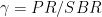
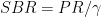
We can also express this range in terms of the contraction (N-x development) or expansion (N+x development) we need in comparison to an average scene with an SBR of 7 stops. If our scene spans more than 7 stops, we need to contract it back to 7, while if our scene spans less than 7 stops we need to expand it. To determine by how much we should do this, we compare the calculated SBR with our reference SBR. In our N+x notation, the value of x is found as 
Although these graphs include a wealth of information, they are not practical to use in the field. For this we convert our values into graphs, and use interpolation to find the values corresponding to intermediate development times that we haven’t tested. The first representation of the data is shown in Figure 4, where we plot the average gradient as a function of development time. For interpolation purposes I have included second order polynomial functions that fit rather well in this case.

More useful in practice are the graphs that relate the subject brightness range to the required development time, either in terms of N+x (Figure 5) or SBR (Figure 6). In both cases I have used splines to connect the data points for interpolation. I recommend that you calibrate the horizontal axis in half stops or one third stops accurate for easy use. Anything more precise will proof unnecessary in the field.


Based on Figure 5, we can interpolate the values for intermediate subject brightness ranges and find the corresponding development time. This is especially useful in your darkroom. If you mark your negatives with the used N+x exposure, the table will directly give you the required development time.
| N+x | Development time (mm:ss) | N+x | Development time (mm:ss) | N+x | Development time (mm:ss) |
| -2 | 03:55 | 0 | 05:45 | 2 | 09:45 |
| -1 2/3 | 04:15 | 1/3 | 06:15 | 2 1/3 | 10:50 |
| -1 1/2 | 04:25 | 1/2 | 06:30 | 2 1/2 | 11:45 |
| -1 1/3 | 04:30 | 2/3 | 06:45 | 2 2/3 | 13:10 |
| -1 | 04:45 | 1 | 07:25 | 3 | 16:25 |
| – 2/3 | 05:00 | 1 1/3 | 08:15 | ||
| – 1/2 | 05:15 | 1 1/2 | 08:25 | ||
| – 1/3 | 05:25 | 1 2/3 | 08:50 | ||
Finding the exposure index (effective film speed)
The previous sections only told half off the story: given a certain scene and exposure, we can now obtain the corresponding development time and we are left with the required exposure. For this we need to determine the effective exposure index (EI) that we will use on our light meter. The value we choose depends on the subject brightness range.
The method proposed by Davis in Beyond the Zone System locates the value of log E that corresponds to the ISO sensitivity. In his book, Davis explains a method of doing this graphically, but I rather use the fact that the value of log E varies smoothly with the average gradient. The ISO standard differs from the standard we use here, and uses a SBR of 1.3 instead of 2.1 and a PR of 0.8 instead of 1.2. It uses a IDmin value in accordance with Davis of 0.1 over B+F. This effectively translates into a gradient of 0.62. If we plot the values of log E at IDmin versus the corresponding gradient from Table 2, we can estimate the value for log E at IDmin for this gradient. In this case we find a value of approximately 0.44. The required graph can be found in Figure 7.

The found value of log E at IDmin corresponds to the box speed of the film, which in the case of Ilford FP4+ is ISO 125. The exposure index corresponding to other values of log E at IDmin can be found using 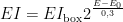


In Way Beyond Monochrome, Lambrecht and Woodhouse favour a more pragmatic approach that requires an additional exposure. The camera is focused at infinity and the frame is filled with a large gray card. Several exposures are then made in which the gray card is “placed” at zone I.5 (underexposed by 3.5 stops with respect to the meter reading) for several exposure indices. After development the resulting density of all exposures is measured. The exposure index that yields a density closest to IDmin = 0.17 is used as a reference to calculate the exposure indices corresponding to the other curves. In the book, Lambrecht and Woodhouse use a sheet per exposure. This is rather wasteful and requires up to 10 sheets. I also made several costly attempts at this, but found that fluctuations in the light conditions between several sheets are large enough to ruin the accuracy of the test. Instead, you can also use the step wedge and clamp it to the film as a variable density filter as shown in Figure 8. This way you only need to make one exposure.

To make the exposure, make sure to use a large and diffuse light source (window light on an overcast day for example). The setup I used is depicted in Figure 9. The exposure variation across the gray card was within 0.2 stops. I suggest you make the exposure using an exposure index of twice the box speed. Every step in the strip than gives you approximately 1/2 stop of reduction in exposure index. For better results you can use the measured densities of the test strip and use the fact that 0.30 log density corresponds to 1 stop of light.

I unfortunately forgot to double the exposure index and illuminated the film at box speed. This time I got lucky and the required value of 0.17 log density was covered by the measured values. The results are presented in Figure 10. As you can read from the graph, the required density corresponds to an estimated exposure index of 140. This is within 1/6 stop of the box speed of 125 and falls within the accuracy on the test.

The exposure indices resulting from the two methods are shown in Figure 11. As can be seen in the graph the constant density approach of Way Beyond Monochrome results in lower exposure indices. In other words, a longer exposure is required. In this case, however the difference between the two methods is less than a half stop in the worst case and both serve as a good starting point.

Comparing with a rule-of-thumb
To put the results in perspective, lets have a look at the rule of thumb proposed by Lambrecht and Woodhouse: for low contrast scenes (rainy or foggy days) stick to the box speed and the suggested development time, for a scene of normal contrast (bright but cloudy day) reduce the effective film speed by 2/3rd stop and the development time by 15%, and for a high contrast scene (bright and sunny day) reduce the film speed by 1 1/3rd stop in total and bring the developing time back by 30%. For your reference, I have summarized the resulting film speeds in Table 4 below. The listed speeds are rounded to the closest film speed setting available on conventional cameras and light meters.
| Box speed | Low contrast | Normal contrast | High contrast |
|---|---|---|---|
| 25 | 25 | 16 | 10 |
| 50 | 50 | 32 | 20 |
| 100 | 100 | 64 | 40 |
| 125 | 125 | 80 | 50 |
| 200 | 200 | 125 | 80 |
| 320 | 320 | 200 | 125 |
| 400 | 400 | 250 | 160 |
| 800 | 800 | 500 | 320 |
| 1600 | 1600 | 1000 | 640 |
| 3200 | 3200 | 2000 | 1250 |
| Development time | Nominal | -15 % | -30 % |
These guidelines are nothing more than a realization of the age-old rule: “Expose for the shadows and develop for the highlights.” The higher the contrast of the scene, the harder it becomes to capture the full range from shadows to highlights. By lowering the exposure index, we are effectively overexposing the film to bring in more shadow detail. By reducing the development time, the highlights are kept from developing too much density. Judging by the actual exposure indices used by many people, this seems to be accurate enough for most users and offers at least a very decent starting point. For the example of this article, the rule of thumb suggests that EI 80 will be good first bet for FP4+. The test, however, suggests we can use box speed for scenes of normal contrast. This is due to the choice for Ilford DD-X as developer. DD-X is known as ‘full speed developer’, and has no or little loss in effective film speed. Lambrecht and Woodhouse tested FP4+ for their methods using ID-11 1:1 and did find a reduction in exposure index.
The log exposure range (LER), a.k.a., matching the negatives to the paper
Photo paper responds to light in a very similar fashion as film does, but at much tighter limits. Where for modern films we typically only get to work with the toe and the linear parts of the density-exposure curve, paper also has a shoulder area: the regime where additional exposure does not result in further darkening of the paper. The maximum density reached we name Dmax. Just as film has a base+fog density, so does paper. We call this minimum density (measured after development) Dmin. When we print a negative onto the paper, we do not want our important information to end up in the print as either Dmin or Dmax, because no detail would be visible. Therefore we define a minimum image density IDmin of Dmin + 0.04 and a maximum image density at 90% of Dmax. The difference between the relative exposures required to reach IDmin and IDmax is called the textural log exposure range (LER).
Papers are manufactured in several contrast grades with corresponding LERs to cope with negatives of different contrasts. According to the ISO standards of 1992, the paper LERs corresponding to specific paper grades is summarized in Table 5. You may remember that before we assumed a pictorial range of 1.2 and a paper grade 2. The LER for paper grade 2 is, however, 1.05. We allow some of the more extreme zones to bleed into the toe and shoulder parts of the curve.
| ISO paper grade | 0 | 1 | 2 | 3 | 4 | 5 |
| LER | 1.55 | 1.28 | 1.05 | 0.88 | 0.73 | 0.58 |
When using variable contrast paper, the story gets slightly more complex. The filter numbers do not correspond to ISO paper grades. For example, Ilford MGIV filter number 2 leans more towards ISO grade 3 and 2, while Kodak VC filter 2 leans more towards ISO grade 1. The effective LER depends on the age of the paper, the age of your colour filters, colour spectrum of your light source (which changes over time) and optics. If you really want to fine tune this, you will have to do a test similar to the one described here to test the response of the paper.
How to use this in the field
After reading this article you may wonder how to use this wealth of information in the field? Luckily, we only need 1 table for this. In the field you have to go through the following steps:
- Measure the subject brightness range and make a note of it.
- Find the corresponding exposure index in Table 6.
- Measure the exposure for the shadow that still needs to register detail. Place it in zone I.5 by subtracting 3.5 stops from the meter reading.
- Correct the exposure time for bellows extension and reciprocity failure if necessary and expose.
- Back in the darkroom, find the development time corresponding to the subject brightness range in Table 6.
- Develop accordingly. Stick to the test conditions as close as possible.
| WBM | BTZS | |||
| N+x | EI | Development time | EI | Development time |
| -2 | 220 | 04:05 | 230 | 03:55 |
| -1 2/3 | 210 | 04:20 | 220 | 04:15 |
| -1 1/2 | 190 | 04:25 | 195 | 04:25 |
| -1 1/3 | 175 | 04:30 | 175 | 04:30 |
| -1 | 170 | 04:40 | 170 | 04:45 |
| – 2/3 | 160 | 05:00 | 160 | 05:00 |
| – 1/2 | 150 | 05:05 | 150 | 05:15 |
| – 1/3 | 135 | 05:10 | 135 | 05:25 |
| 0 | 130 | 05:35 | 130 | 05:45 |
| 1/3 | 125 | 06:05 | 130 | 06:15 |
| 1/2 | 115 | 06:20 | 120 | 06:30 |
| 2/3 | 105 | 06:35 | 115 | 06:45 |
| 1 | 100 | 07:20 | 115 | 07:25 |
| 1 1/3 | 95 | 08:10 | 115 | 08:15 |
| 1 1/2 | 90 | 08:35 | 110 | 08:25 |
| 1 2/3 | 85 | 09:05 | 110 | 08:50 |
| 2 | 80 | 10:20 | 110 | 09:45 |
| 2 1/3 | 80 | 12:20 | 105 | 10:50 |
| 2 1/2 | 75 | 13:50 | 105 | 11:45 |
| 2 2/3 | 75 | 15:25 | 100 | 13:10 |
| 3 | 100 | 16:15 | ||
Conclusions
Using the methods described above we can calibrate our development times and exposure index to achieve complete control over our negative densities and contrast. In this specific case I tested Ilford FP4+ in combination with rotary development in Ilford DD-X at a 1:4 dilution. Although the two proposed methods clearly give different results, the difference is not larger than 1/2 stop and both sets of results can be used in practice. Although Variable Contrast papers give us a lot of leeway and possibilities for tuning the contrast in print, fine tuning your film exposure and development are useful for achieving optimal results and for bringing greater technical understanding into your work.
You must be logged in to post a comment.